POPS vs BayesianRidge: Uncertainty for Low-Noise Surrogates

Demonstrates how POPSRegression provides better uncertainty estimates than BayesianRidge when fitting a misspecified model to low-noise data.

In computational science, surrogate models are often fit to near-deterministic data. When the model class cannot exactly reproduce the target function (model misspecification), standard Bayesian regression significantly underestimates predictive uncertainty because it only captures epistemic uncertainty, which vanishes with more data.

POPS Regression corrects this by estimating misspecification uncertainty from pointwise optimal parameter sets. The result is wider, more honest error bars that properly cover the true function.

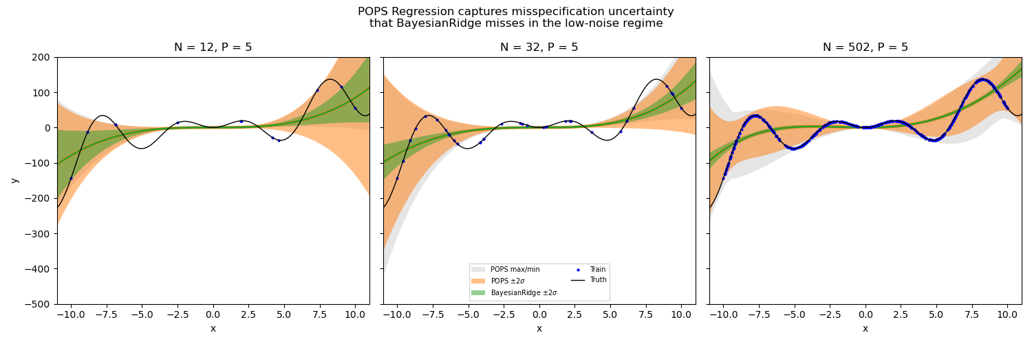
In this example we fit a 4th-degree polynomial to a complex oscillatory function with varying numbers of training points. The green band shows the (too narrow) epistemic-only uncertainty from BayesianRidge, while the orange band shows the POPS uncertainty that accounts for misspecification. The gray region shows the full min/max posterior prediction range.

# Authors: Thomas D Swinburne <tswin@umich.edu>,
#          Danny Perez <danny_perez@lanl.gov>
# SPDX-License-Identifier: BSD-3-Clause

Generate low-noise data from a complex function

We create a target function that a 4th-degree polynomial cannot perfectly reproduce. This is the “misspecification” — the model is structurally unable to capture the true function, regardless of how much data we have.

import numpy as np

rng = np.random.RandomState(42)


def target_function(x):
    return (x**3 + 0.01 * x**4) * 0.1 + np.sin(x) * x * 10.0


x_test = np.linspace(-11, 11, 200)
y_test = target_function(x_test)

Fit models with different training set sizes

We compare POPSRegression and BayesianRidge for N = 10, 30, and 500 training points. As N increases, BayesianRidge epistemic uncertainty shrinks to near-zero, but POPS misspecification uncertainty persists because the polynomial is fundamentally unable to fit the target.

from sklearn.linear_model import BayesianRidge
from sklearn.preprocessing import PolynomialFeatures

from popsregression import POPSRegression

import matplotlib.pyplot as plt

fig, axes = plt.subplots(1, 3, figsize=(15, 5), sharey=True)
train_sizes = [10, 30, 500]

for ax, n_samples in zip(axes, train_sizes):
    # Generate training data (no noise — purely deterministic)
    x_train = np.sort(
        np.append(rng.uniform(-1, 1, n_samples), np.linspace(-1, 1, 2)) * 10
    )
    y_train = target_function(x_train)

    poly = PolynomialFeatures(degree=4, include_bias=True)
    X_train = poly.fit_transform(x_train.reshape(-1, 1))
    X_test = poly.fit_transform(x_test.reshape(-1, 1))

    # POPS Regression
    pops = POPSRegression(resampling_method="sobol", resample_density=10.0)
    pops.fit(X_train, y_train)
    y_pred, y_std, y_max, y_min = pops.predict(
        X_test, return_std=True, return_bounds=True
    )

    # BayesianRidge (epistemic uncertainty only, excluding aleatoric alpha_)
    br = BayesianRidge(fit_intercept=False)
    br.fit(X_train, y_train)
    br_pred = br.predict(X_test)
    br_epistemic_std = np.sqrt(np.sum(np.dot(X_test, br.sigma_) * X_test, axis=1))

    # Plot
    ax.fill_between(
        x_test,
        y_min,
        y_max,
        alpha=0.2,
        facecolor="0.5",
        label="POPS max/min",
    )
    ax.fill_between(
        x_test,
        y_pred - 2 * y_std,
        y_pred + 2 * y_std,
        alpha=0.5,
        facecolor="C1",
        label=r"POPS $\pm 2\sigma$",
    )
    ax.plot(x_test, y_pred, "C1-", lw=3)

    ax.fill_between(
        x_test,
        br_pred - 2 * br_epistemic_std,
        br_pred + 2 * br_epistemic_std,
        alpha=0.5,
        facecolor="C2",
        label=r"BayesianRidge $\pm 2\sigma$",
    )
    ax.plot(x_test, br_pred, "C2-", lw=2)

    ax.plot(x_train, y_train, "b.", ms=4, label="Train")
    ax.plot(x_test, y_test, "k-", lw=1, label="Truth")

    ax.set_ylim(-500, 200)
    ax.set_xlim(-11, 11)
    ax.set_title(f"N = {len(x_train)}, P = {X_train.shape[1]}")
    ax.set_xlabel("x")

axes[0].set_ylabel("y")
axes[1].legend(loc="lower center", fontsize=7, ncol=2)
fig.suptitle(
    "POPS Regression captures misspecification uncertainty\n"
    "that BayesianRidge misses in the low-noise regime",
    fontsize=12,
)
plt.tight_layout()
plt.show()

Key observations

• N = 10: Both methods show wide uncertainty, but POPS (orange) is wider and provides better coverage of the true function (black).

• N = 30: BayesianRidge epistemic uncertainty (green) has already shrunk significantly, while POPS correctly maintains wider bands where the polynomial deviates from the truth.

• N = 500: BayesianRidge epistemic uncertainty is nearly invisible, yet the polynomial still cannot match the oscillatory target. POPS maintains honest uncertainty that reflects this structural limitation.

This demonstrates the core insight: for low-noise misspecified models, adding more data does not reduce the true parameter uncertainty — it only reduces the epistemic component. POPS captures the remaining misspecification component that standard Bayesian regression ignores.

Comparing posterior types

POPSRegression supports two posterior forms: 'hypercube' (default) and 'ensemble'.

fig, axes = plt.subplots(1, 2, figsize=(12, 5), sharey=True)
posteriors = ["ensemble", "hypercube"]

n_samples = 30
x_train = np.sort(
    np.append(rng.uniform(-1, 1, n_samples), np.linspace(-1, 1, 2)) * 10
)
y_train = target_function(x_train)

poly = PolynomialFeatures(degree=4, include_bias=True)
X_train = poly.fit_transform(x_train.reshape(-1, 1))
X_test = poly.fit_transform(x_test.reshape(-1, 1))

for ax, posterior in zip(axes, posteriors):
    pops = POPSRegression(
        posterior=posterior,
        resampling_method="uniform",
        resample_density=10.0,
        leverage_percentile=0.0,
    )
    pops.fit(X_train, y_train)
    y_pred, y_std, y_max, y_min = pops.predict(
        X_test, return_std=True, return_bounds=True
    )

    ax.fill_between(
        x_test, y_min, y_max, alpha=0.2, facecolor="0.5", label="max/min"
    )
    ax.fill_between(
        x_test,
        y_pred - 2 * y_std,
        y_pred + 2 * y_std,
        alpha=0.5,
        facecolor="C1",
        label=r"$\pm 2\sigma$",
    )
    ax.plot(x_test, y_pred, "C1-", lw=3)
    ax.plot(x_train, y_train, "b.", ms=6, label="Train")
    ax.plot(x_test, y_test, "k-", lw=1, label="Truth")

    ax.set_ylim(-500, 200)
    ax.set_xlim(-11, 11)
    ax.set_title(f"posterior = '{posterior}'")
    ax.set_xlabel("x")

axes[0].set_ylabel("y")
axes[0].legend(loc="lower center", fontsize=8)
fig.suptitle("Comparison of POPS posterior types (N=30)", fontsize=12)
plt.tight_layout()
plt.show()

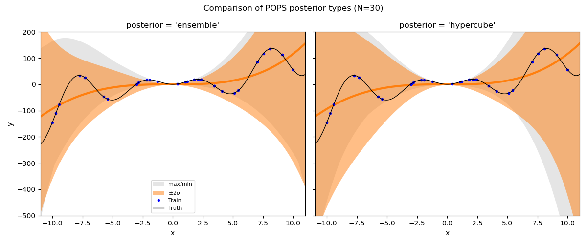
The 'hypercube' posterior (default) tends to give the most conservative bounds, while 'ensemble' directly uses the pointwise corrections.